Kirchhoff’s current and voltage laws

In our last article, we looked at the principles and operation of a d.c motor.  In this article, we’re going to investigate Kirchoff’s current and voltage laws, as well as how to apply them to engineering problems.

Kirchoff’s law of  current

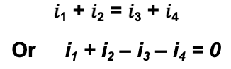
Kirchoff’s law of current states that the algebraic sum of all current at any node in an electrical circuit is equal to zero or the sum of the currents flowing into a node is equal to the sum of the currents flowing out of that node.

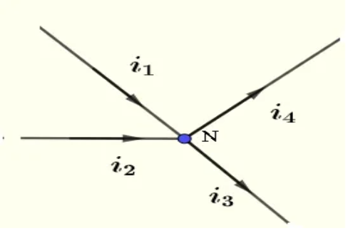
At the node N above, we write:

Kirchoff’s law of voltage

Kirchoff’s law of voltage states that in any closed loop in an electrical circuit, the algebraic sum of all voltages around the loop is equal to zero.

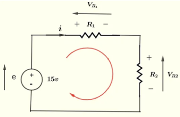
Using the closed loop, we may write:

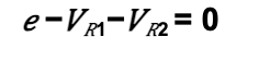
Since the voltages across the resistors are in the opposite direction to the e.m.f of the cell. 

Electromotive force e.m.f and internal resistance

The electromotive force (e) or e.m.f is the energy provided by a cell or battery per coulomb of charge passing through it, and it’s measured in volts V.

It’s equal to the potential difference across the terminal of the cell when no current is flowing:

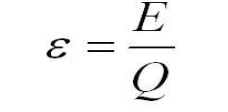
• ꜫ = electromotive force in volts, V
• E = energy in joules, J
• Q = charge in coulombs, C

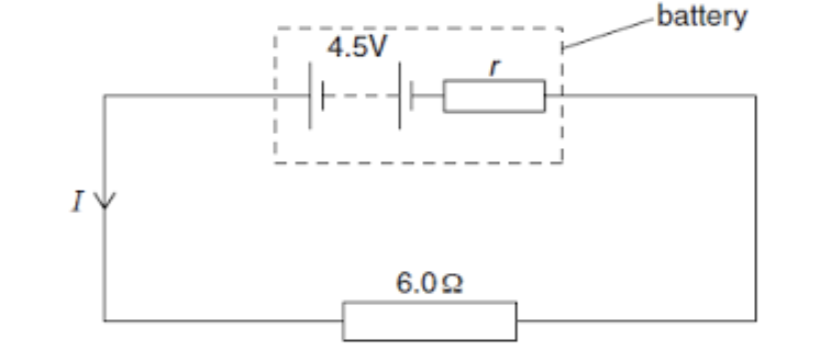
Batteries and cells have an internal resistance (r) which is measured in ohm’s (Ω). When electricity flows around a circuit the internal resistance of the cell itself resists the flow of current and so thermal (heat) energy is wasted in the cell itself.

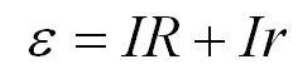
Ohms law is then expanded to include this internal resistance

• ꜫ = electromotive force in volts, V
• I = current in amperes, A
• R = resistance of the load in the circuit in ohms, Ω
• r = internal resistance of the cell in ohms, Ω

We can rearrange the above equation;

and then to

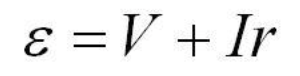
In this equation (V) appears which is the terminal potential difference, measured in volts (V). 

The potential difference across the terminals of the cell when current is flowing in the circuit is always less than the e.m.f. of the cell.

We can also calculate the e.m.f from a graph of V against I.  If we plot a graph of terminal potential difference (V) against the current in the circuit (I) we get a straight line with a negative gradient.

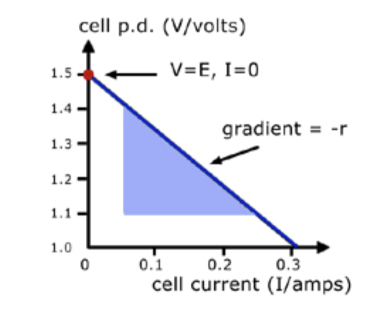
We can then rearrange the e.m.f. equation from above to match the general expression for 

a straight line, y = mx +c.

If we start with ꜫ = V + Ir 

Rearrange to make V the subject: V = -Ir + ꜫ

Compare this to Y = mx + c (typical equation for a straight line graph)

We can see that the gradient = – r and the intercept = ꜫ

Interested in our courses?

You can read more about our selection of accredited online electrical engineering courses here.

Check out individual courses pages below:

Diploma in Electrical and Electronic Engineering

Higher International Certificate in Electrical and Electronic Engineering

Diploma in Electrical Technology

Diploma in Electronics

Diploma in Renewable Energy (Electrical)

Higher International Diploma in Electrical and Electronic EngineeringAlternatively, you can view all our online engineering courses here.