How can we analyse a single-degree-of-freedom lumped parameter system with damping?
In our previous article on undamped vibration, we looked at solving vibration problems with a single degree of freedom. In this article, we’re going to look at systems with damping and how to analyse them.
We’ll focus on the mathematical analysis of a single-degree-of-freedom lumped parameter system with damping.
Damped Single Degree of Freedom
Think about an experiment like Hooke’s Law, this time we plot V vs. velocity:
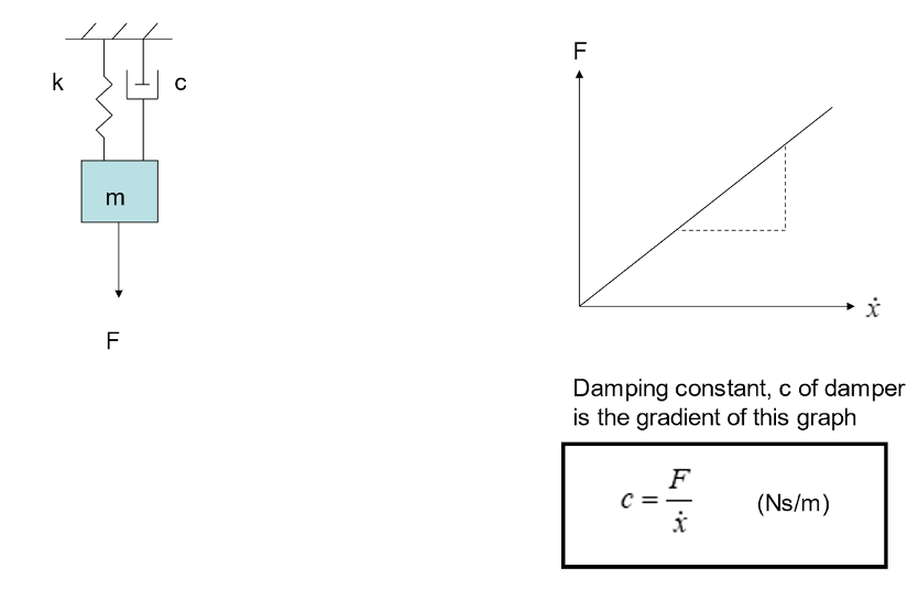
The damping constant, c, is analogous to the spring constant, k. The difference is that the force is proportional to velocity, whereas that force was proportional to displacement for a spring previously.
If we think about the damped system in equilibrium and then analyse the forces acting on the mass in a FBD, we can obtain the equation of motion via Newton’s second law:
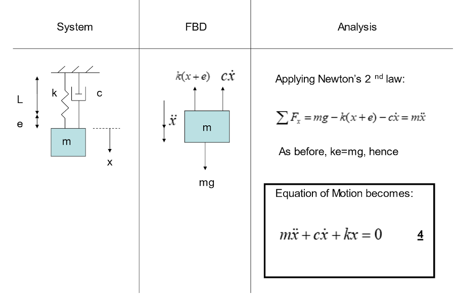
The equation of motion here is like that of an undamped system, with the addition of an extra term to account for the damping in this model.
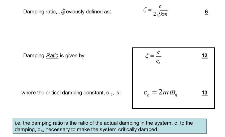
If we divide through the equation by the mass, known as normalising, we get an alternative form of the equation of motion, as you can see in the image below. This normalised version of the equation of motion can be used to infer model parameters of the system, such as the undamped natural frequency and the damping ratio.
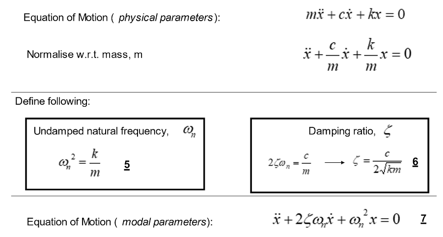
These model parameters are distinct from the physical parameters of the system. It’s possible to describe the equation of motion either in physical or modal parameters with no loss or duplication of information.
Response to damping
So, let’s think about the response of the system to various amounts of damping. The damping ration can be under damped, over damped, or critically damped:
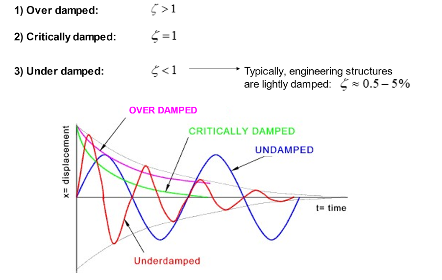
Critical damping is the reference case; damping in the system means there is no overshoot in the response. In other words, the system decays to zero without passing the equilibrium position.
Typically, most engineering structures are lightly damped and have a damping ratio value in the single figures as a percentage. Here, there is overshoot followed by several oscillations before the system comes to rest:
Damped Natural Frequency and Damped Time Period
The inclusion of damping in a system has the effect of reducing the resonance frequency slightly, which is said to occur at the damped natural frequency, d, given by: d=n1-2
Now, as it is typically ~ 0.5–5%, then for light damping: dn
The time is also slightly modified and is referred to as the damped time, Td,: Td = 1fd = 2πd.
Finally, the time solution for the damped SDOF system can be summarised as < 1 and c < cc. If we assume that t = 0 and the displacement, x = A when the mass is released, we get a decaying cosinusoidal oscillation. The displacement is described by the following equation:.
x=Ae-ξntcos(dt)
Example
Let’s look at an example to see how this works in real life. Take a mass of 4kg that is suspended on a spring with a stiffness of 3000 N/m. The system is fitted with a damper, with a damping ration of 0.2. The mass is pulled down to 50mm and then released.
Firstly, we want to calculate the damped natural frequency. We can do this through this equation:
n=km=30004=27.4 rad/s
d=n1-2
d=27.41-0.22=26.8 rad/s
Then we want to calculate the displacement after 0.5 seconds. The initial displacement = 25mm, which is 0.025m. So therefore:
x=Ae-ξntcos(dt)
x=0.025e-(0.2) (27.4) (0.5) cos ({26.8} {0.5})
x=0.025e-(2.74) cos (13.4)
x=0.0250.0650.67=1.08×10⁻³ m
x=1.08 mm
Let’s imagine we have a railroad system that we are working on. The bumper is designed as a spring and viscous damper in parallel with one another. We want to find out the bumper’s damping constant, with a damping ration of 1.25, when the bumper is engaged by a railroad car weighing 20,000kg and that has a stiffness of 2×10⁵ N/m.
To do this, we can use this equation:
n=km=2×10520000=3.16 rad/s
c=2ξnm
c=21.253.1620000
c=158113=158 kNs/m
Ok, now let’s imagine an empty railroad car with a mass of 4,500kg. We want to find the undamped natural frequency and the damping ratio when engaged to an empty railroad car:
n=km=2×1054500=6.6 rad/s
c=2ξnm
ξ=c2nm
ξ=1581132(6.6) (4500)
ξ=2.63=263%
This is the last of our articles on damping and vibrations but keep an eye out for more exciting engineering articles on various topics.
Interested in our courses?
Interested in civil or mechanical engineering? Find out more about all the civil engineering courses we have available by clicking here, and the mechanical engineering courses by clicking here.
Diploma in Mechanical Engineering
Diploma in Mechanical Technology
Diploma in Sustainable Construction
Diploma in Structural Engineering
Diploma in Building and Construction Engineering
Higher International Certificate in Civil Engineering
Higher International Diploma in Civil Engineering
Higher International Diploma in Mechanical Engineering
Higher International Certificate in Mechanical Engineering
Alternatively, you can view all our online engineering courses here.
Recent Posts
Essential Formulas for Calculating Drilling Parameters
Essential Formulas for Calculating Drilling Parameters When it comes to precision and efficiency in manufacturing, few processes are as foundational—or as critical—as drilling. Whether you’re a seasoned engineer or a student entering the world of mechanical or industrial engineering, understanding how to correctly calculate drilling parameters can significantly impact the quality of your work, the […]
From Raw Material to Refined Component: The Role of Drilling and Turning
From Raw Material to Refined Component: The Role of Drilling and Turning Secondary processes are used in manufacturing to further modify the output of primary manufacturing processes in order to improve the material properties, surface quality, surface integrity, appearance and dimensional tolerance. In this blog, we will focus on drilling and turning as secondary manufacturing […]
Behind the Cutter: How Milling Shapes the Future of Manufacturing
Behind the Cutter: How Milling Shapes the Future of Manufacturing Secondary processes are used in manufacturing to further modify the output of primary manufacturing processes in order to improve the material properties, surface quality, surface integrity, appearance and dimensional tolerance. In this blog, we will focus on milling as a secondary manufacturing process. Machining refers […]

